Steel is usually defined as an alloy of iron and carbon with the carbon content between a few hundreds of a percent up to about 2 wt%. Other alloying elements can amount in total to about 5 wt% in low-alloy steels and higher in more highly alloyed steels such as tool steels, stainless steels (>10.5%) and heat resisting CrNi steels (>18%). Steels can exhibit a wide variety of properties depending on composition as well as the phases and micro-constituents present, which in turn depend on the heat treatment.
The Fe-C Phase Diagram
The basis for the understanding of the heat treatment of steels is the Fe-C phase diagram (Fig 1). Figure 1 actually shows two diagrams; the stable iron-graphite diagram (dashed lines) and the metastable Fe-Fe3C diagram. The stable condition usually takes a very long time to develop, especially in the low-temperature and low-carbon range, and therefore the metastable diagram is of more interest. The Fe-C diagram shows which phases are to be expected at equilibrium (or metastable equilibrium) for different combinations of carbon concentration and temperature.
We distinguish at the low-carbon end ferrite (α-iron),which can at most dissolve 0.028% C, at 727°C (1341°F) and austenite -iron, which can dissolve 2.11 wt% C at 1148°C (2098°F). At the carbon-rich side we find cementite (Fe3C). Of less interest, except for highly alloyed steels, is the δ-ferrite existing at the highest temperatures.
Between the single-phase fields are found regions with mixtures of two phases, such as ferrite + cementite, austenite + cementite, and ferrite + austenite. At the highest temperatures, the liquid phase field can be found and below this are the two phase fields liquid + austenite, liquid + cementite, and liquid + δ-ferrite.
In heat treating of steels, the liquid phase is always avoided. Some important boundaries at single-phase fields have been given special names:
- A1, the so-called eutectoid temperature, which is the minimum temperature for austenite
- A3, the lower-temperature boundary of the austenite region at low carbon contents, that is, the γ/γ + α boundary
- Acm, the counterpart boundary for high carbon contents, that is, the γ/γ + Fe3C boundary
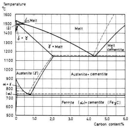
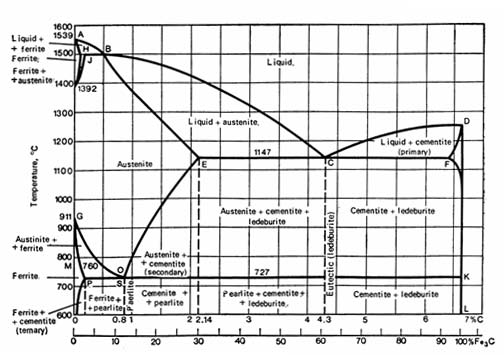
Fig. 1. The Fe-Fe3C diagram.
The Fe-C diagram in Fig 1 is of experimental origin. The knowledge of the thermodynamic principles and modern thermodynamic data now permits very accurate calculations of this diagram. This is particularly useful when phase boundaries must be extrapolated and at low temperatures where the experimental equilibria are extremely slow to develop.
If alloying elements are added to the iron-carbon alloy (steel), the position of the A1, A3, and Acm boundaries and the eutectoid composition are changed. It suffices here to mention that
- all important alloying elements decrease the eutectoid carbon content,
- the austenite-stabilizing elements manganese and nickel decrease A, and
- the ferrite-stabilizing elements chromium, silicon, molybdenum, and tungsten increase A1.
Transformation Diagrams
The kinetic aspects of phase transformations are as important as the equilibrium diagrams for the heat treatment of steels. The metastable phase martensite and the morphologically metastable microconstituent bainite, which are of extreme importance to the properties of steels, can generally form with comparatively rapid cooling to ambient temperature. That is when the diffusion of carbon and alloying elements is suppressed or limited to a very short range.
Bainite is a eutectoid decomposition that is a mixture of ferrite and cementite. Martensite, the hardest constituent, forms during severe quenches from supersaturated austenite by a shear transformation. Its hardness increases monotonically with carbon content up to about 0.7 wt%. If these unstable metastable products are subsequently heated to a moderately elevated temperature, they decompose to more stable distributions of ferrite and carbide. The reheating process is sometimes known as tempering or annealing.
The transformation of an ambient temperature structure like ferrite-pearlite or tempered martensite to the elevated-temperature structure of austenite or austenite-carbide is also of importance in the heat treatment of steel.
One can conveniently describe what is happening during transformation with transformation diagrams. Four different types of such diagrams can be distinguished. These include:
- Isothermal transformation diagrams describing the formation of austenite, which will be referred to as ITh diagrams
- Isothermal transformation (IT) diagrams, also referred to as time-temperature-transformation (TTT) diagrams, describing the decomposition of austenite
- Continuous heating transformation (CRT) diagrams
- Continuous cooling transformation (CCT) diagrams
Isothermal Transformation Diagrams
This type of diagram shows what happens when a steel is held at a constant temperature for a prolonged period. The development of the microstructure with time can be followed by holding small specimens in a lead or salt bath and quenching them one at a time after increasing holding times and measuring the amount of phases formed in the microstructure with the aid of a microscope.
ITh Diagrams (Formation of Austenite). During the formation of austenite from an original microstructure of ferrite and pearlite or tempered martensite, the volume decreases with the formation of the dense austenite phase. From the elongation curves, the start and finish times for austenite formation, usually defined as 1% and 99% transformation, respectively, can be derived.
IT Diagrams (Decomposition of Austenite). The procedure starts at a high temperature, normally in the austenitic range after holding there long enough to obtain homogeneous austenite without undissolved carbides, followed by rapid cooling to the desired hold temperature. The cooling was started from 850°C (1560°F). The A1 and A3 temperatures are indicated as well as the hardness. Above A3 no transformation can occur. Between A1 and A3 only ferrite can form from austenite.
CRT Diagrams
In practical heat treatment situations, a constant temperature is not required, but rather a continuous changing temperature during either cooling or heating. Therefore, more directly applicable information is obtained if the diagram is constructed from dilatometric data using a continuously increasing or decreasing temperature.
Like the ITh diagrams, the CRT diagrams are useful in predicting the effect of short-time austenitization that occurs in induction and laser hardening. One typical question is how high the maximum surface temperature should be in order to achieve complete austenitization for a given heating rate. To high a temperature may cause unwanted austenite grain growth, which produces a more-brittle martensitic microstructure.
CCT Diagrams
As for heating diagrams, it is important to clearly state what type of cooling curve the transformation diagram was derived from.
Use of a constant cooling rate is very common in experimental practice. However, this regime rarely occurs in a practical situation. One can also find curves for so-called natural cooling rates according to Newton’s law of cooling. These curves simulate the behavior in the interior of a large part such as the cooling rate of a Jominy bar at some distance from the quenched end.
Close to the surface the characteristics of the cooling rare can be very complex. Each CCT diagram contains a family of curves representing the cooling rates at different depths of a cylinder with a 300 mm (12 in.) diameter. The slowest cooling rate represents the center of the cylinder. The more severe the cooling medium, the longer the times to which the C-shaped curves are shifted. The M, temperature is unaffected.
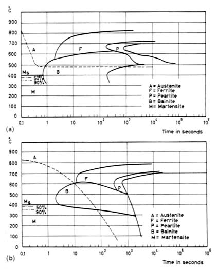
Fig.2. CCT (a) and TTT (b) diagrams.
It should be noted, however, that transformation diagrams can not be used to predict the response to thermal histories that are very much different from the ones used to construct the diagrams. For instance, first cooling rapidly to slightly above Ms and then reheating to a higher temperature will give more rapid transformation than shown in the IT diagram because nucleation is greatly accelerated during the introductory quench. It should also be remembered that the transformation diagrams are sensitive to the exact alloying content within me allowable composition range.
List of Articles - Knowledge Base