A typical stress-strain curve is shown in Figure 1. If we begin from the origin and follow the graph a number of points are indicated.
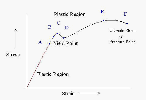
Figure 1: A typical stress-strain curve
Point A: At origin, there is no initial stress or strain in the test piece. Up to point A Hooke's Law is obeyed according to which stress is directly proportional to strain. That's why the point A is also known as proportional limit. This straight line region is known as elastic region and the material can regain its original shape after removal of load.
Point B: The portion of the curve between AB is not a straight line and strain increases faster than stress at all points on the curve beyond point A. Point B is the point after which any continuous stress results in permanent, or inelastic deformation. Thus, point B is known as the elastic limit or yield point.
Point C & D: Beyond the point B, the material goes to the plastic stage till the point C is reached. At this point the cross- sectional area of the material starts decreasing and the stress decreases to point D. At point D the workpiece changes its length with a little or without any increase in stress up to point E.
Point E: Point E indicates the location of the value of the ultimate stress. The portion DE is called the yielding of the material at constant stress. From point E onwards, the strength of the material increases and requires more stress for deformation, until point F is reached.
Point F: A material is considered to have completely failed once it reaches the ultimate stress. The point of fracture, or the actual tearing of the material, does not occur until point F. The point F is also called ultimate point or fracture point.
If the instantaneous minimal cross-sectional area can be measured during a test along with P and L and if the constant-volume deformation assumption is valid while plastic deformation is occurring, then a true stress-strain diagram can be constructed.
The construction should consist of using the equation ε = log (L/L0) for true strain in the elastic and initial plastic regions and the equation ε= log (A0/A) once significant plastic deformation has begun. In practice, however, the equation ε= log (A0/A) is used for the entire strain range since the amount of error introduced is usually negligible. The equation σ = P/A for true stress is valid throughout the entire test.
Accurate construction of a true stress-strain diagram becomes exceedingly difficult if the plastic deformation cannot be assumed to occur at a constant volume.
Finally, it should be mentioned that the neither the true stress-strain diagram nor the engineering stress-strain diagram accounts for the fact that the state of stress within the necked-down region is multiaxial. There is no simple way to account for the effect of this multiaxial state of stress on the material’s response, so it is customarily ignored. A schematic representation of an engineering stress-strain diagram and the corresponding true stress-strain diagram can be found in Figure 2.
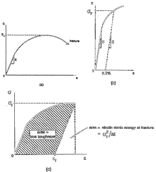
Figure 2: Material properties determined from stress-strain diagrams: (a) Engineering stress-strain diagram; (b) determination σ by the offset method; (c) true stress-strain diagram
The KEY to METALS database brings global metal properties together into one integrated and searchable database. Quick and easy access to the mechanical properties, chemical composition, cross-reference tables, and
more provide users with an unprecedented wealth of information. Click the buttons below to learn more from the Guided Tour or to test drive the KEY to METALS database.